Draw Circle Using Trigonometric Method

Radians

Radians are another manner of measuring angles, and the mensurate of an angle can exist converted betwixt degrees and radians.

Learning Objectives

Explain the definition of radians in terms of arc length of a unit circle and use this to convert between degrees and radians

Central Takeaways

Key Points

• One radian is the measure of the central bending of a circumvolve such that the length of the arc is equal to the radius
  of the circle.
• A total revolution of a circumvolve ([latex]360^{\circ}[/latex]) equals [latex]ii\pi~\mathrm{radians}[/latex]. This ways that [latex]\displaystyle{ one\text{ radian} = \frac{180^{\circ}}{\pi} }[/latex]. [latex][/latex]
• The formula used to convert betwixt radians and degrees is [latex]\displaystyle{ \text{angle in degrees} = \text{angle in radians} \cdot \frac{180^\circ}{\pi} }[/latex].
• The radian measure of an angle is the ratio of the length of the arc to the radius of the circle [latex]\displaystyle{ \left(\theta = \frac{southward}{r}\right) }[/latex]. In other words, if [latex]s[/latex] is the length of an arc of a circle, and [latex]r[/latex] is the radius of the circumvolve, then the cardinal angle containing that arc measures radians.

Fundamental Terms

• arc: A continuous office of the circumference of a circle.
• circumference: The length of a line that bounds a circumvolve.
• radian: The standard unit used to measure out angles in mathematics. The measure of a central angle of a circle that intercepts an arc equal in length to the radius of that circle.

Introduction to Radians

Recall that dividing a circle into 360 parts creates the degree measurement. This is an arbitrary measurement, and we may choose other ways to divide a circle. To find some other unit of measurement, think of the process of drawing a circle. Imagine that you stop before the circle is completed. The portion that y'all drew is referred to as an arc. An arc may be a portion of a total circle, a full circle, or more a full circumvolve, represented past more than one full rotation. The length of the arc around an entire circle is called the circumference of that circumvolve.

The circumference of a circle is

[latex]C = ii \pi r[/latex]

If nosotros split both sides of this equation by [latex]r[/latex], we create the ratio of the circumference, which is e'er [latex]ii\pi[/latex] to the radius, regardless of the length of the radius. And so the circumference of any circle is [latex]2\pi \approx 6.28[/latex] times the length of the radius. That ways that if we took a string as long equally the radius and used it to measure consecutive lengths around the circumference, there would be room for six full cord-lengths and a little more than a quarter of a seventh, every bit shown in the diagram below.

The circumference of a circle compared to the radius: The circumference of a circle is a footling more than six times the length of the radius.

This brings us to our new angle mensurate. The radian is the standard unit used to measure angles in mathematics. I radian is the mensurate of a central angle of a circle that intercepts an arc equal in length to the radius of that circle.

I radian: The angle [latex]t[/latex] sweeps out a measure of one radian. Note that the length of the intercepted arc is the same as the length of the radius of the circumvolve.

Because the full circumference of a circle equals [latex]2\pi[/latex] times the radius, a full circular rotation is [latex]ii\pi[/latex] radians.

Radians in a circle: An arc of a circumvolve with the same length as the radius of that circle corresponds to an angle of i radian. A total circle corresponds to an angle of [latex]2\pi[/latex] radians; this ways that[latex]2\pi[/latex] radians is the same as [latex]360^\circ[/latex].

Note that when an angle is described without a specific unit, it refers to radian measure. For example, an bending measure out of iii indicates three radians. In fact, radian measure is dimensionless, since it is the quotient of a length (circumference) divided by a length (radius), and the length units cancel. You may sometimes see radians represented by the symbol [latex]\text{rad}[/latex].

Comparing Radians to Degrees

Since we now know that the full range of a circle can be represented past either 360 degrees or [latex]2\pi[/latex] radians, we tin can conclude the following:

[latex]\displaystyle{ \brainstorm{align} 2\pi \text{ radians} &= 360^{\circ} \\ 1\text{ radian} &= \frac{360^{\circ}}{2\pi} \\ 1\text{ radian} &= \frac{180^{\circ}}{\pi} \end{align}}[/latex]

Equally stated, ane radian is equal to [latex]\displaystyle{ \frac{180^{\circ}}{\pi} }[/latex] degrees, or just under 57.3 degrees ([latex]57.three^{\circ}[/latex]). Thus, to convert from radians to degrees, we tin can multiply by [latex]\displaystyle{ \frac{180^\circ}{\pi} }[/latex]:

[latex]\displaystyle{ \text{bending in degrees} = \text{angle in radians} \cdot \frac{180^\circ}{\pi} }[/latex]

A unit circle is a circle with a radius of i, and it is used to show certain mutual angles.

Unit circle: Commonly encountered angles measured in radians and degrees.

Example

Catechumen an angle measuring [latex]\displaystyle{ \frac{\pi}{9} }[/latex] radians to degrees.

Substitute the bending in radians into the in a higher place formula:

[latex]\displaystyle{ \begin{marshal} \text{angle in degrees} &= \text{angle in radians} \cdot \frac{180^\circ}{\pi} \\ \text{angle in degrees} &= \frac{\pi}{nine} \cdot \frac{180^\circ}{\pi} \\ &=\frac{180^{\circ}}{9} \\ &= twenty^{\circ} \cease{marshal} }[/latex]

Thus nosotros have [latex]\displaystyle{ \frac{\pi}{9} \text{ radians} = 20^{\circ} }[/latex].

Measuring an Angle in Radians

An arc length [latex]s[/latex] is the length of the curve along the arc. Just as the full circumference of a circumvolve ever has a constant ratio to the radius, the arc length produced by any given angle also has a constant relation to the radius, regardless of the length of the radius.

This ratio, called the radian measure, is the same regardless of the radius of the circumvolve—it depends only on the bending. This property allows us to define a measure of whatsoever angle as the ratio of the arc length [latex]southward[/latex] to the radius [latex]r[/latex].

[latex]\displaystyle{ \begin{marshal} due south &= r \theta \\ \theta &= \frac{s}{r} \finish{align} }[/latex]

Measuring radians: (a) In an bending of 1 radian; the arc lengths equals the radius [latex]r[/latex]. (b) An bending of 2 radians has an arc length [latex]s=2r[/latex]. (c) A full revolution is [latex]2\pi[/latex], or near 6.28 radians.

Example

What is the measure of a given bending in radians if its arc length is [latex]four \pi[/latex], and the radius has length [latex][/latex]12?

Substitute the values [latex]due south = four\pi[/latex] and [latex]r = 12[/latex] into the angle formula:

[latex]\displaystyle{ \brainstorm{align} \theta &= \frac{south}{r} \\ & = \frac{4\pi}{12} \\ &= \frac{\pi}{3} \\ &= \frac{1}{3}\pi \end{align} }[/latex]

The bending has a measure of [latex]\displaystyle{\frac{1}{3}\pi}[/latex] radians.

Defining Trigonometric Functions on the Unit Circle

Identifying points on a unit circumvolve allows i to utilise trigonometric functions to any angle.

Learning Objectives

Use right triangles drawn in the unit circle to define the trigonometric functions for whatsoever angle

Fundamental Takeaways

Central Points

• The [latex]10[/latex]– and [latex]y[/latex]-coordinates at a point on the unit of measurement circle given by an angle [latex]t[/latex] are divers by the functions [latex]x = \cos t[/latex] and [latex]y = \sin t[/latex].
• Although the tangent part is not indicated by the unit of measurement circle, we can apply the formula [latex]\displaystyle{\tan t = \frac{\sin t}{\cos t}}[/latex] to find the tangent of any bending identified.
• Using the unit circle, nosotros are able to apply trigonometric functions to whatever angle, including those greater than [latex]xc^{\circ}[/latex].
• The unit circle demonstrates the periodicity of trigonometric functions by showing that they result in a repeated ready of values at regular intervals.

Cardinal Terms

• periodicity: The quality of a role with a repeated set of values at regular intervals.
• unit circumvolve: A circumvolve centered at the origin with radius 1.
• quadrants: The four quarters of a coordinate plane, formed by the [latex]ten[/latex]– and [latex]y[/latex]-axes.

Trigonometric Functions and the Unit Circle

We have already defined the trigonometric functions in terms of right triangles. In this section, we will redefine them in terms of the unit circle. Recollect that a unit circle is a circle centered at the origin with radius i. The bending [latex]t[/latex] (in radians ) forms an arc of length [latex]s[/latex].

The x- and y-axes divide the coordinate plane (and the unit circumvolve, since it is centered at the origin) into four quarters called quadrants. We label these quadrants to mimic the management a positive bending would sweep. The iv quadrants are labeled I, II, Three, and IV.

For whatever bending [latex]t[/latex], we tin can label the intersection of its side and the unit of measurement circumvolve by its coordinates, [latex](x, y)[/latex]. The coordinates [latex]x[/latex] and [latex]y[/latex] volition be the outputs of the trigonometric functions [latex]f(t) = \cos t[/latex] and [latex]f(t) = \sin t[/latex], respectively. This means:

[latex]\displaystyle{ \begin{align} x &= \cos t \\ ​y &= \sin t \cease{align} }[/latex]

The diagram of the unit circumvolve illustrates these coordinates.

Unit of measurement circumvolve: Coordinates of a point on a unit circumvolve where the central bending is [latex]t[/latex] radians.

Annotation that the values of [latex]ten[/latex] and [latex]y[/latex] are given by the lengths of the two triangle legs that are colored red. This is a right triangle, and you tin see how the lengths of these two sides (and the values of [latex]ten[/latex] and [latex]y[/latex]) are given past trigonometric functions of [latex]t[/latex].

For an example of how this applies, consider the diagram showing the point with coordinates [latex]\displaystyle{\left(-\frac{\sqrt2}{2}, \frac{\sqrt2}{2}\correct) }[/latex] on a unit circumvolve.

Point on a unit of measurement circumvolve: The point [latex]\displaystyle{ \left(-\frac{\sqrt2}{2}, \frac{\sqrt2}{2}\right) }[/latex] on a unit circle.

We know that, for any betoken on a unit circle, the [latex]x[/latex]-coordinate is [latex]\cos t[/latex] and the [latex]y[/latex]-coordinate is [latex]\sin t[/latex]. Applying this, we can identify that [latex]\displaystyle{\cos t = -\frac{\sqrt2}{2}}[/latex] and  [latex]\displaystyle{\sin t = -\frac{\sqrt2}{2}}[/latex] for the angle [latex]t[/latex] in the diagram.

Recall that [latex]\displaystyle{\tan t = \frac{\sin t}{\cos t}}[/latex].  Applying this formula, we tin detect the tangent of any angle identified past a unit circumvolve equally well. For the angle [latex]t[/latex] identified in the diagram  of the unit circle showing the signal [latex]\displaystyle{\left(-\frac{\sqrt2}{2}, \frac{\sqrt2}{two}\right)}[/latex], the tangent is:

[latex]\displaystyle{\begin{align}\tan t &= \frac{\sin t}{\cos t} \\&= \frac{-\frac{\sqrt2}{ii}}{-\frac{\sqrt2}{ii}} \\&= ane\end{marshal}}[/latex]

We take previously discussed trigonometric functions as they utilise to right triangles. This allowed the states to brand observations about the angles and sides of right triangles, but these observations were limited to angles with measures less than [latex]90^{\circ}[/latex]. Using the unit circle, we are able to apply trigonometric functions to angles greater than [latex]90^{\circ}[/latex].

Farther Consideration of the Unit Circle

The coordinates of sure points on the unit circumvolve and the the mensurate of each angle in radians and degrees are shown in the unit of measurement circle coordinates diagram. This diagram allows ane to brand observations about each of these angles using trigonometric functions.

Unit circle coordinates: The unit circumvolve, showing coordinates and angle measures of certain points.

We can find the coordinates of any point on the unit circle. Given whatever angle [latex]t[/latex], we can find the [latex]x[/latex]– or [latex]y[/latex]-coordinate at that point using [latex]x = \text{cos } t[/latex]  and [latex]y = \text{sin } t[/latex].

The unit of measurement circle demonstrates the periodicity of trigonometric functions. Periodicity refers to the manner trigonometric functions result in a repeated set of values at regular intervals. Take a look at the [latex]x[/latex]-values of the coordinates in the unit of measurement circle above for values of [latex]t[/latex] from [latex]0[/latex] to [latex]2{\pi}[/latex]:

[latex]{1, \frac{\sqrt{3}}{2}, \frac{\sqrt{ii}}{2}, \frac{ane}{two}, 0, -\frac{i}{2}, -\frac{\sqrt{ii}}{2}, -\frac{\sqrt{three}}{2}, -ane, -\frac{\sqrt{3}}{ii}, -\frac{\sqrt{two}}{2}, -\frac{1}{2}, 0, \frac{1}{2}, \frac{\sqrt{2}}{2}, \frac{\sqrt{3}}{2}, 1}[/latex]

We can identify a pattern in these numbers, which fluctuate betwixt [latex]-1[/latex] and [latex]1[/latex]. Note that this blueprint will repeat for higher values of [latex]t[/latex]. Retrieve that these [latex]10[/latex]-values represent to [latex]\cos t[/latex]. This is an indication of the periodicity of the cosine part.

Case

Solve [latex]\displaystyle{ \sin{ \left(\frac{7\pi}{6}\right) } }[/latex].

It seems similar this would be complicated to work out. Notwithstanding, detect that the unit circle diagram shows the coordinates at [latex]\displaystyle{ t = \frac{7\pi}{6} }[/latex]. Since the [latex]y[/latex]-coordinate corresponds to [latex]\sin t[/latex], we can identify that

[latex]\displaystyle{\sin{ \left(\frac{7\pi}{6}\right)} = -\frac{1}{2} }[/latex]

Special Angles

The unit of measurement circle and a ready of rules tin be used to recollect the values of trigonometric functions of special angles.

Learning Objectives

Explicate how the properties of sine, cosine, and tangent and their signs in each quadrant requite their values for each of the special angles

Key Takeaways

Key Points

• The trigonometric functions for the angles in the unit circumvolve can be memorized and recalled using a set of rules.
• The sign on a trigonometric role depends on the quadrant that the angle falls in, and the mnemonic phrase "A Smart Trig Class" is used to place which functions are positive in which quadrant.
• Reference angles in quadrant Iare used to place which value any angle in quadrants II, III, or Iv will take. A reference angle forms the same bending with the [latex]x[/latex]-axis as the angle in question.
• Just the sine and cosine functions for special angles are included in the unit circle. All the same, since tangent is derived from sine and cosine, it tin be calculated for any of the special angles.

Primal Terms

• special angle: An angle that is a multiple of thirty or 45 degrees; trigonometric functions are easily written at these angles.

Trigonometric Functions of Special Angles

Retrieve that certain angles and their coordinates, which correspond to [latex]x = \cos t[/latex] and [latex]y = \sin t[/latex] for a given angle [latex]t[/latex], can exist identified on the unit of measurement circle.

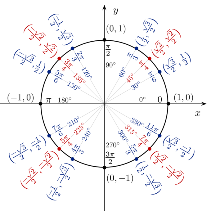
Unit circle: Special angles and their coordinates are identified on the unit circumvolve.

The angles identified on the unit circle higher up are called special angles; multiples of [latex]\pi[/latex], [latex]\frac{\pi}{two}[/latex], [latex][/latex][latex]\frac{\pi}{iii}[/latex], [latex]\frac{\pi}{4}[/latex], and [latex]\frac{\pi}{half-dozen}[/latex] ([latex]180^\circ[/latex][latex][/latex], [latex]ninety^\circ[/latex], [latex]60^\circ[/latex],  [latex]45^\circ[/latex], and [latex]30^\circ[/latex]). These take relatively elementary expressions. Such simple expressions generally do non exist for other angles. Some examples of the algebraic expressions for the sines of special angles are:

[latex]\displaystyle{ \brainstorm{align} \sin{\left( 0^{\circ} \correct)} &= 0 \\ \sin{\left( xxx^{\circ} \correct)} &= \frac{i}{2} \\ \sin{\left( 45^{\circ} \right)} &= \frac{\sqrt{2}}{ii} \\ \sin{\left( 60^{\circ} \right)} &= \frac{\sqrt{3}}{two} \\ \sin{\left( ninety^{\circ} \right)} &= i \\ \end{align} }[/latex]

The expressions for the cosine functions of these special angles are also simple.

Annotation that while but sine and cosine are divers directly by the unit circumvolve, tangent can be defined as a quotient involving these two:

[latex]\displaystyle{ \tan t = \frac{\sin t}{\cos t} }[/latex]

Tangent functions likewise have simple expressions for each of the special angles.

We can discover this trend through an instance. Let's observe the tangent of [latex]lx^{\circ}[/latex].

Showtime, we can identify from the unit circle that:

[latex]\displaystyle{ \brainstorm{marshal} \sin{ \left(threescore^{\circ}\right) } &= \frac{\sqrt{iii}}{two} \\ \cos{ \left(60^{\circ}\right) } &= \frac{1}{two} \end{marshal} }[/latex]

We tin can easily calculate the tangent:

[latex]\displaystyle{ \begin{align} \tan{\left(sixty^{\circ}\right)} &= \frac{\sin{\left(60^{\circ}\right)}}{\cos{\left(sixty^{\circ}\right)}} \\ &= \frac{\frac{\sqrt{3}}{ii}}{\frac{ane}{2}} \\ &= \frac{\sqrt{three}}{2} \cdot \frac{2}{ane} \\ &= \sqrt{three} \stop{align} }[/latex]

Memorizing Trigonometric Functions

An agreement of the unit circle and the ability to quickly solve trigonometric functions for certain angles is very useful in the field of mathematics. Applying rules and shortcuts associated with the unit of measurement circle allows you to solve trigonometric functions quickly. The following are some rules to help you apace solve such problems.

Signs of Trigonometric Functions

The sign of a trigonometric role depends on the quadrant that the angle falls in. To help remember which of the trigonometric functions are positive in each quadrant, we can use the mnemonic phrase "A Smart Trig Course." Each of the 4 words in the phrase corresponds to one of the four quadrants, starting with quadrant I and rotating counterclockwise. In quadrant I, which is "A," all of the trigonometric functions are positive. In quadrant II, "Smart," simply sine is positive. In quadrant III, "Trig," only tangent is positive. Finally, in quadrant IV, "Class," only cosine is positive.

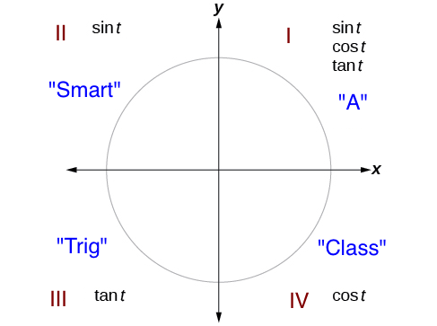
Sign rules for trigonometric functions: The trigonometric functions are each listed in the quadrants in which they are positive.

Identifying Values Using Reference Angles

Take a close await at the unit circle, and note that [latex]\sin t[/latex] and [latex]\cos t[/latex] accept certain values as they fluctuate betwixt [latex]-one[/latex] and [latex]ane[/latex]. Y'all volition find that they take on the value of zero, likewise as the positive and negative values of three detail numbers: [latex]\displaystyle{\frac{\sqrt{three}}{ii}}[/latex], [latex]\displaystyle{\frac{\sqrt{2}}{two}}[/latex], and [latex]\displaystyle{\frac{1}{2}}[/latex]. Identifying reference angles volition assist us place a pattern in these values.

Reference angles in quadrant I are used to identify which value any bending in quadrants 2, Iii, or 4 volition take. This means that nosotros merely demand to memorize the sine and cosine of three angles in quadrant I: [latex]30^{\circ}[/latex], [latex]45^{\circ}[/latex], and [latex]60^{\circ}[/latex].

For whatsoever given bending in the get-go quadrant, at that place is an angle in the 2d quadrant with the same sine value. Because the sine value is the [latex]y[/latex]-coordinate on the unit of measurement circle, the other angle with the same sine will share the same [latex]y[/latex]-value, but take the contrary [latex]x[/latex]-value. Therefore, its cosine value volition be the opposite of the first bending'due south cosine value.

Likewise, there will be an angle in the fourth quadrant with the same cosine as the original angle. The angle with the same cosine volition share the aforementioned [latex]x[/latex]-value just will accept the reverse [latex]y[/latex]-value. Therefore, its sine value will exist the contrary of the original angle'due south sine value.

As shown in the diagrams beneath, angle [latex]\alpha[/latex] has the same sine value equally angle [latex]t[/latex]; the cosine values are opposites. Angle [latex]\beta[/latex] has the same cosine value as bending [latex]t[/latex]; the sine values are opposites.

[latex]\displaystyle{ \begin{align} \sin t = \sin \blastoff \quad &\text{and} \quad \cos t = -\cos \alpha \\ \sin t = -\sin \beta \quad &\text{and} \quad \cos t = \cos \beta \terminate{align} }[/latex]

Reference angles: In the left figure, [latex]t[/latex] is the reference angle for [latex]\alpha[/latex]. In the right figure, [latex]t[/latex] is the reference angle for [latex]\beta[/latex].

Remember that an bending'south reference bending is the acute angle, [latex]t[/latex], formed by the terminal side of the angle [latex]t[/latex] and the horizontal axis. A reference bending is e'er an angle between [latex]0[/latex] and [latex]90^{\circ}[/latex], or [latex]0[/latex] and [latex]\displaystyle{\frac{\pi}{two}}[/latex] radians. For whatsoever bending in quadrants Two, III, or IV, there is a reference bending in quadrant I.

Reference angles in each quadrant: For any angle in quadrants 2, Three, or IV, there is a reference angle in quadrant I.

Thus, in guild to call up any sine or cosine of a special angle, you lot need to be able to identify its angle with the [latex]x[/latex]-axis in club to compare it to a reference bending. Y'all will and so identify and apply the appropriate sign for that trigonometric part in that quadrant.

These are the steps for finding a reference angle for any angle betwixt [latex]0[/latex] and [latex]2\pi[/latex]:

1. An bending in the offset quadrant is its own reference bending.
2. For an angle in the second or tertiary quadrant, the reference angle is [latex]|\pi - t|[/latex] or [latex]|180^{\circ} - t|[/latex].
3. For an bending in the fourth quadrant, the reference angle is [latex]2\pi - t[/latex] or [latex]360^{\circ} - t[/latex]. If an angle is less than [latex]0[/latex] or greater than [latex]2\pi[/latex], add or subtract [latex]2\pi[/latex] equally many times every bit needed to find an equivalent angle between [latex]0[/latex] and [latex]2\pi[/latex].

Since tangent functions are derived from sine and cosine, the tangent can be calculated for whatever of the special angles by first finding the values for sine or cosine.

Example

Detect [latex]\tan (225^{\circ})[/latex], applying the rules above.

Kickoff, note that [latex]225^{\circ}[/latex] falls in the tertiary quadrant:

Bending [latex]225^{\circ}[/latex] on a unit circle: The bending [latex]225^{\circ}[/latex]falls in quadrant Iii.

Subtract [latex]225^{\circ}[/latex] from [latex]180^{\circ}[/latex] to identify the reference angle:

[latex]\displaystyle{ \begin{align} \left| 180^{\circ} - 225^{\circ} \right| &= \left|-45^{\circ} \right| \\ &= 45^{\circ} \cease{marshal} }[/latex]

In other words, [latex]225^{\circ}[/latex] falls [latex]45^{\circ}[/latex] from the [latex]x[/latex]-axis. The reference angle is [latex]45^{\circ}[/latex].

Recall that

[latex]\displaystyle{\sin{ \left(45^{\circ}\right)} = \frac{\sqrt{2}}{ii} }[/latex]

Nonetheless, the rules described above tell united states of america that the sine of an angle in the 3rd quadrant is negative. And so we have

[latex]\displaystyle{\sin{ \left(225^{\circ}\correct)} = -\frac{\sqrt{ii}}{2} }[/latex]

Post-obit the same process for cosine, we can identify that

[latex]\displaystyle{ \cos{ \left(225^{\circ}\right)} = -\frac{\sqrt{ii}}{2} }[/latex]

We can detect [latex]\tan (225^{\circ})[/latex] by dividing [latex]\sin (225^{\circ})[/latex] past [latex]\cos (225^{\circ})[/latex]:

[latex]\displaystyle{ \begin{marshal} \tan{ \left(225^{\circ}\correct)} &= \frac{\sin(225^{\circ})}{\cos (225^{\circ})} \\ &= \frac{-\frac{\sqrt{2}}{2}}{-\frac{\sqrt{ii}}{2}} \\ &= -\frac{\sqrt{two}}{2} \cdot -\frac{ii}{\sqrt{two}} \\ &= 1 \end{align} }[/latex]

Sine and Cosine equally Functions

The functions sine and cosine can be graphed using values from the unit circle, and certain characteristics tin exist observed in both graphs.

Learning Objectives

Describe the characteristics of the graphs of sine and cosine

Key Takeaways

Central Points

• Both the sine role [latex](y = \sin x)[/latex] and cosine function [latex](y = \cos ten)[/latex] can be graphed past plotting points derived from the unit circumvolve, with each [latex]ten[/latex]-coordinate being an angle in radians and the [latex]y[/latex]-coordinate being the corresponding value of the role at that angle.
• Sine and cosine are periodic functions with a period of [latex]two\pi[/latex].
• Both sine and cosine have a domain of [latex](-\infty, \infty)[/latex] and a range of [latex][-i, 1][/latex].
• The graph of [latex]y = \sin x[/latex] is symmetric about the origin because it is an odd function, while the graph of [latex]y = \cos x[/latex] is symmetric about the [latex]y[/latex]-axis because it is an fifty-fifty function.

Key Terms

• period: An interval containing values that occur repeatedly in a function.
• fifty-fifty office: A continuous set of [latex]\left(x,f(10)\right)[/latex] points in which [latex]f(-ten) = f(10)[/latex], with symmetry about the [latex]y[/latex]-axis.
• odd function: A continuous set of [latex]\left(ten, f(x)\right)[/latex] points in which [latex]f(-10) = -f(10)[/latex], with symmetry near the origin.
• periodic function: A continuous set up of [latex]\left(x,f(x)\correct)[/latex] points that repeats at regular intervals.

Graphing Sine and Cosine Functions

Recall that the sine and cosine functions chronicle real number values to the [latex]x[/latex]– and [latex]y[/latex]-coordinates of a indicate on the unit circumvolve. So what practise they wait like on a graph on a coordinate plane? Permit'due south kickoff with the sine function, [latex]y = \sin x[/latex]. We can create a tabular array of values and use them to sketch a graph. Below are some of the values for the sine function on a unit circumvolve, with the [latex]x[/latex]-coordinate being the angle in radians and the [latex]y[/latex]-coordinate being [latex]\sin 10[/latex]:

[latex]\displaystyle{ (0, 0) \quad (\frac{\pi}{vi}, \frac{1}{ii}) \quad (\frac{\pi}{4}, \frac{\sqrt{two}}{2}) \quad (\frac{\pi}{iii}, \frac{\sqrt{3}}{two}) \quad (\frac{\pi}{ii}, 1) \\ (\frac{two\pi}{iii}, \frac{\sqrt{3}}{ii}) \quad (\frac{3\pi}{iv}, \frac{\sqrt{two}}{2}) \quad (\frac{v\pi}{6}, \frac{1}{two}) \quad (\pi, 0) }[/latex]

Plotting the points from the table and continuing along the [latex]x[/latex]-axis gives the shape of the sine function.

Graph of the sine function: Graph of points with [latex]x[/latex] coordinates existence angles in radians, and [latex]y[/latex] coordinates being the function [latex]\sin ten[/latex].

Notice how the sine values are positive betwixt [latex]0[/latex] and [latex]\pi[/latex], which stand for to the values of the sine function in quadrants I and II on the unit of measurement circumvolve, and the sine values are negative between [latex]\pi[/latex] and [latex]2\pi[/latex], which correspond to the values of the sine function in quadrants 3 and Iv on the unit circle.

Plotting values of the sine office: The points on the curve [latex]y = \sin x[/latex] correspond to the values of the sine function on the unit circumvolve.

Now permit'south have a like await at the cosine role, [latex]f(ten) = \sin x[/latex]. Again, we can create a table of values and use them to sketch a graph. Below are some of the values for the sine function on a unit circle, with the [latex]x[/latex]-coordinate beingness the bending in radians and the [latex]y[/latex]-coordinate being [latex]\cos x[/latex]:

[latex]\displaystyle{ (0, ane) \quad (\frac{\pi}{half-dozen}, \frac{\sqrt{iii}}{2}) \quad (\frac{\pi}{iv}, \frac{\sqrt{two}}{ii}) \quad (\frac{\pi}{3}, \frac{i}{2}) \quad (\frac{\pi}{2}, 0) \\ (\frac{two\pi}{3}, -\frac{one}{ii}) \quad (\frac{3\pi}{4}, -\frac{\sqrt{2}}{2}) \quad (\frac{five\pi}{half-dozen}, -\frac{\sqrt{3}}{2}) \quad (\pi, -1) }[/latex]

Every bit with the sine part, nosotros can plots points to create a graph of the cosine function.

Graph of the cosine function: The points on the curve [latex]y = \cos 10[/latex] represent to the values of the cosine function on the unit circle.

Considering we tin can evaluate the sine and cosine of any real number, both of these functions are defined for all real numbers. By thinking of the sine and cosine values equally coordinates of points on a unit circle, it becomes clear that the range of both functions must be the interval [latex]\left[-1, 1 \right][/latex].

Identifying Periodic Functions

In the graphs for both sine and cosine functions, the shape of the graph repeats after [latex]2\pi[/latex], which means the functions are periodic with a menstruum of [latex]2\pi[/latex]. A periodic function is a function with a repeated set of values at regular intervals. Specifically, it is a function for which a specific horizontal shift, [latex]P[/latex], results in a function equal to the original function:

[latex]f(x + P) = f(x)[/latex]

for all values of [latex]x[/latex] in the domain of [latex]f[/latex]. When this occurs, nosotros call the smallest such horizontal shift with [latex]P>0[/latex] the period of the function. The diagram below shows several periods of the sine and cosine functions.

Periods of the sine and cosine functions: The sine and cosine functions are periodic, significant that a specific horizontal shift, [latex]P[/latex], results in a function equal to the original function:[latex]f(ten + P) = f(10)[/latex].

Even and Odd Functions

Looking once more at the sine and cosine functions on a domain centered at the [latex]y[/latex]-axis helps reveal symmetries. As we can see in the graph of the sine function, it is symmetric about the origin, which indicates that information technology is an odd office. All along the graph, whatsoever two points with opposite [latex]x[/latex] values likewise have contrary [latex]y[/latex] values. This is characteristic of an odd role: ii inputs that are opposites have outputs that are besides opposites. In other words, if [latex]\sin (-x) = - \sin x[/latex].

Odd symmetry of the sine function: The sine function is odd, meaning it is symmetric well-nigh the origin.

The graph of the cosine function shows that information technology is symmetric well-nigh the y-axis. This indicates that it is an even function. For even functions, any two points with opposite [latex]10[/latex]-values have the same office value. In other words, [latex]\cos (-x) = \cos x[/latex]. Nosotros can see from the graph that this is true by comparing the [latex]y[/latex]-values of the graph at any reverse values of [latex]x[/latex].

Even symmetry of the cosine function: The cosine function is even, significant it is symmetric about the [latex]y[/latex]-axis.

Tangent as a Function

Characteristics of the tangent function can be observed in its graph.

Learning Objectives

Describe the characteristics of the graph of the tangent function

Key Takeaways

Cardinal Points

• The tangent role is undefined at any value of [latex]ten[/latex] where [latex]\cos ten = 0[/latex], and its graph has vertical asymptotes at these [latex]x[/latex] values.
• Tangent is a periodic function with a flow of [latex]\pi[/latex].
• The graph of the tangent part is symmetric around the origin, and thus is an odd office.

Central Terms

• periodic function: A continuous set of [latex]\left(x, f(x)\correct)[/latex] points with a set of values that repeats at regular intervals.
• menstruation: An interval containing the minimum set of values that echo in a periodic office.
• odd function: An continuous ready of [latex]\left(x, f(x)\right)[/latex] points in which [latex]f(-10) = -f(x)[/latex], and there is symmetry about the origin.
• vertical asymptote: A direct line parallel to the [latex]y[/latex] centrality that a curve approaches arbitrarily closely as the curve goes to infinity.

Graphing the Tangent Function

The tangent function can be graphed by plotting [latex]\left(x,f(10)\right)[/latex]  points. The shape of the office can be created past finding the values of the tangent at special angles. Withal, it is not possible to observe the tangent functions for these special angles with the unit circle. We utilize the formula, [latex]\displaystyle{ \tan x = \frac{\sin 10}{\cos 10} }[/latex] to make up one's mind the tangent for each value.

We can analyze the graphical beliefs of the tangent role past looking at values for some of the special angles. Consider the points below, for which the [latex]ten[/latex]-coordinates are angles in radians, and the [latex]y[/latex]-coordinates are [latex]\tan x[/latex]:

[latex]\displaystyle{ (-\frac{\pi}{2}, \text{undefined}) \quad (-\frac{\pi}{3}, -\sqrt{three}) \quad (-\frac{\pi}{4}, -1) \quad (-\frac{\pi}{6}, -\frac{\sqrt{iii}}{three}) \quad (0, 0) \\ (\frac{\pi}{half dozen}, \frac{\sqrt{3}}{3}) \quad (\frac{\pi}{iv}, 1) \quad (\frac{\pi}{three}, \sqrt{iii}) \quad (\frac{\pi}{2}, \text{undefined}) }[/latex]

Notice that [latex]\tan ten[/latex] is undefined at [latex]\displaystyle{x = -\frac{\pi}{2}}[/latex] and [latex]\displaystyle{x = \frac{\pi}{two}}[/latex]. The above points will help us draw our graph, but we demand to determine how the graph behaves where it is undefined. Let's consider the last four points. We can identify that the values of [latex]y[/latex] are increasing as [latex]x[/latex] increases and approaches [latex]\displaystyle{\frac{\pi}{2}}[/latex]. Nosotros could consider boosted points betwixt [latex]\displaystyle{x=0}[/latex] and [latex]\displaystyle{x = \frac{\pi}{2}}[/latex], and we would meet that this holds. Likewise, we can meet that [latex]y[/latex] decreases equally [latex]x[/latex] approaches [latex]\displaystyle{-\frac{\pi}{2}}[/latex], because the outputs get smaller and smaller.

Recall that in that location are multiple values of [latex]x[/latex] that tin can give [latex]\cos 10 = 0[/latex]. At any such point, [latex]\tan x[/latex] is undefined because [latex]\displaystyle{\tan 10 = \frac{\sin x}{\cos 10}}[/latex]. At values where the tangent function is undefined, there are discontinuities in its graph. At these values, the graph of the tangent has vertical asymptotes.

Graph of the tangent function: The tangent function has vertical asymptotes at [latex]\displaystyle{10 = \frac{\pi}{2}}[/latex] and [latex]\displaystyle{x = -\frac{\pi}{2}}[/latex].

Characteristics of the Graph of the Tangent Function

Every bit with the sine and cosine functions, tangent is a periodic function. This means that its values repeat at regular intervals. The menstruum of the tangent function is [latex]\pi[/latex] because the graph repeats itself on [latex]10[/latex]-centrality intervals of [latex]chiliad\pi[/latex], where [latex]k[/latex] is a abiding. In the graph of the tangent function on the interval [latex]\displaystyle{-\frac{\pi}{2}}[/latex] to [latex]\displaystyle{\frac{\pi}{two}}[/latex], nosotros can see the behavior of the graph over one complete cycle of the function. If we wait at
any larger interval, we will see that the characteristics of the graph repeat.

The graph of the tangent function is symmetric around the origin, and thus is an odd function. In other words, [latex]\text{tan}(-ten) = - \text{tan } x[/latex] for any value of [latex]x[/latex]. Any two points with opposite values of [latex]x[/latex] produce opposite values of [latex]y[/latex]. We can meet that this is true by considering the [latex]y[/latex] values of the graph at whatsoever contrary values of [latex]x[/latex]. Consider [latex]\displaystyle{10=\frac{\pi}{iii}}[/latex] and [latex]\displaystyle{ten=-\frac{\pi}{3}}[/latex]. We already determined above that [latex]\displaystyle{\tan (\frac{\pi}{3}) = \sqrt{3}}[/latex], and [latex]\displaystyle{\tan (-\frac{\pi}{three}) = -\sqrt{3}}[/latex].

Secant and the Trigonometric Cofunctions

Trigonometric functions accept reciprocals that tin exist calculated using the unit circle.

Learning Objectives

Calculate values for the trigonometric functions that are the reciprocals of sine, cosine, and tangent

Key Takeaways

Key Points

• The secant office is the reciprocal of the cosine part [latex]\displaystyle{\left(\sec x = \frac{i}{\cos x}\right)}[/latex]. It can exist found for an angle [latex]t[/latex] by using the [latex]ten[/latex]-coordinate of  the associated bespeak on the unit circle: [latex]\displaystyle{\sec t = \frac{1}{x}}[/latex].
• The cosecant function is the reciprocal of the sine function [latex]\displaystyle{\left(\csc x = \frac{1}{\sin x}\right)}[/latex]. Information technology can be found for an angle [latex]t[/latex] by using the [latex]y[/latex]-coordinate of  the associated bespeak on the unit circle: [latex]\displaystyle{\csc t = \frac{1}{y}}[/latex].
• The cotangent office is the reciprocal of the tangent function [latex]\displaystyle{\left(\cot 10 = \frac{i}{\tan x} = \frac{\cos t}{\sin t}\right)}[/latex]. It can be found for an bending past using the [latex]x[/latex]– and [latex]y[/latex]-coordinates of  the associated betoken on the unit circle: [latex]\displaystyle{\cot t = \frac{\cos t}{\sin t} = \frac{x}{y}}[/latex].

Key Terms

• secant: The reciprocal of the cosine office
• cosecant: The reciprocal of the sine function
• cotangent: The reciprocal of the tangent function

Introduction to Reciprocal Functions

We have discussed three trigonometric functions: sine, cosine, and tangent. Each of these functions has a reciprocal function, which is divers by the reciprocal of the ratio for the original trigonometric function. Notation that reciprocal functions differ from changed functions. Inverse functions are a way of working backwards, or determining an angle given a trigonometric ratio; they involve working with the aforementioned ratios as the original office.

The iii reciprocal functions are described below.

Secant

The secant function is the reciprocal of the cosine function, and is abbreviated as [latex]\sec[/latex].
It tin can be described as the ratio of the length of the hypotenuse to the length of the adjacent side in a triangle.

[latex]\displaystyle{ \begin{align} \sec x &= \frac{ane}{\cos x} \\ \sec x &= \frac{\text{hypotenuse}}{\text{adjacent}} \end{align} }[/latex]

Information technology is easy to calculate secant with values in the unit of measurement circle. Recollect that for any point on the circumvolve, the [latex]x[/latex]-value gives [latex]\cos t[/latex] for the associated angle [latex]t[/latex]. Therefore, the secant role for that angle is

[latex]\displaystyle{\sec t = \frac{1}{x}}[/latex]

Cosecant

The cosecant function is the reciprocal of the sine function, and is abbreviated every bit[latex]\csc[/latex]. Information technology can be described as the ratio of the length of the hypotenuse to the length of the opposite side in a triangle.

[latex]\displaystyle{ \begin{align} \csc 10 &= \frac{ane}{\sin x} \\ \csc x &= \frac{\text{hypotenuse}}{\text{opposite}} \end{align} }[/latex]

Equally with secant, cosecant tin be calculated with values in the unit circle. Retrieve that for whatever point on the circle, the [latex]y[/latex]-value gives [latex]\sin t[/latex]. Therefore, the cosecant function for the same angle is

[latex]\displaystyle{\csc t = \frac{1}{y}}[/latex]

Cotangent

The cotangent part is the reciprocal of the tangent function, and is abbreviated as [latex]\cot[/latex]. Information technology can be described as the ratio of the length of the adjacent side to the length of the hypotenuse in a triangle.

[latex]\displaystyle{ \brainstorm{align} \cot x &= \frac{i}{\tan 10} \\ \cot x &= \frac{\text{next}}{\text{reverse}} \cease{marshal} }[/latex]

Also note that because [latex]\displaystyle{\tan 10 = \frac{\sin x}{\cos ten}}[/latex], its reciprocal is

[latex]\displaystyle{\cot x = \frac{\cos 10}{\sin x}}[/latex]

Cotangent can also be calculated with values in the unit circumvolve. Applying the [latex]x[/latex]– and [latex]y[/latex]-coordinates associated with angle [latex]t[/latex], we have

[latex]\displaystyle{ \begin{align} \cot t &= \frac{\cos t}{\sin t} \\ \cot t &= \frac{ten}{y} \end{align} }[/latex]

Computing Reciprocal Functions

We now recognize six trigonometric functions that can be calculated using values in the unit circle. Think that nosotros used values for the sine and cosine functions to calculate the tangent function. Nosotros will follow a similar process for the reciprocal functions, referencing the values in the unit circle for our calculations.

For example, let's notice the value of [latex]\sec{\left(\frac{\pi}{3}\correct)}[/latex].

Applying [latex]\displaystyle{\sec x = \frac{i}{\cos x}}[/latex], we tin can rewrite this as:

[latex]\displaystyle{ \sec{\left(\frac{\pi}{3}\right)}= \frac{i}{\cos{\left({\frac{\pi}{3}}\right)}} }[/latex]

From the unit circumvolve, we know that [latex]\displaystyle{\cos{\left({\frac{\pi}{3}}\right)}= \frac{1}{two}}[/latex]. Using this, the value of [latex]\displaystyle{ \sec{\left(\frac{\pi}{3}\right)}}[/latex] can be institute:

[latex]\displaystyle{ \begin{align} \sec{\left(\frac{\pi}{3}\right)} &= \frac{1}{\frac{1}{2}} \\ &= 2 \end{marshal} }[/latex]

The other reciprocal functions tin be solved in a similar fashion.

Case

Utilise the unit circumvolve to calculate [latex]\sec t[/latex], [latex]\cot t[/latex], and [latex]\csc t[/latex] at the point [latex]\displaystyle{\left(-\frac{\sqrt{three}}{two}, \frac{1}{2}\right)}[/latex].

Indicate on a unit circle: The point [latex]\displaystyle{\left(-\frac{\sqrt{3}}{2}, \frac{1}{two}\right)}[/latex], shown on a unit circumvolve.

Because we know the [latex](x, y)[/latex] coordinates of the point on the unit of measurement circle indicated by angle [latex]t[/latex], we can use those coordinates to notice the three functions.

Recall that the [latex]ten[/latex]-coordinate gives the value for the cosine function, and the [latex]y[/latex]-coordinate gives the value for the sine function. In other words:

[latex]\displaystyle{ \brainstorm{align} x &= \cos t \\ &= -\frac{\sqrt{3}}{ii} \end{align} }[/latex]

and

[latex]\displaystyle{ \begin{align} y &= \sin t \\ &= \frac{1}{ii} \end{align} }[/latex]

Using this data, the values for the reciprocal functions at bending [latex]t[/latex] tin can exist calculated:

[latex]\displaystyle{ \begin{align} \sec t &= \frac{1}{\cos t} \\ &= \frac{1}{x} \\ &= \left(\frac{i}{-\frac{\sqrt{3}}{2}} \right)\\ &= -\frac{2}{\sqrt{iii}} \\ &= \left(-\frac{2}{\sqrt{3}} \cdot \frac{\sqrt{three}}{\sqrt{3}} \right)\\ &= -\frac{2\sqrt{three}}{3} \finish{align} }[/latex]

[latex]\displaystyle{ \begin{align} \cot t &= \frac{\cos t}{\sin t} \\ &= \frac{10}{y} \\ &= \left(\frac{-\frac{\sqrt{iii}}{2}}{\frac{1}{2}}\right) \\ &= \left(-\frac{\sqrt{3}}{2}\cdot \frac{2}{ane} \correct) \\ &= -\sqrt{3} \terminate{align} }[/latex]

[latex]\displaystyle{ \begin{marshal} \csc t &= \frac{1}{\sin t} \\ & = \frac{i}{y} \\ & = \left(\frac{i}{\frac{1}{ii}}\right) \\ & = 2 \terminate{marshal} }[/latex]

Inverse Trigonometric Functions

Each trigonometric function has an changed role that tin can be graphed.

Learning Objectives

Describe the characteristics of the graphs of the inverse trigonometric functions, noting their domain and range restrictions

Key Takeaways

Key Points

• The inverse function of sine is arcsine, which has a domain of [latex]\displaystyle{\left[-\frac{\pi}{2}, \frac{\pi}{2}\correct]}[/latex]. In other words, for angles in the interval [latex]\displaystyle{\left[-\frac{\pi}{ii}, \frac{\pi}{2}\correct]}[/latex], if [latex]y = \sin x[/latex], and so [latex]\arcsin x = \sin^{−ane} x=y[/latex].
• The inverse part of cosine is arccosine, which has a domain of [latex]\left[0, \pi\right][/latex]. In other words, for angles in the interval [latex]\left[0, \pi\right][/latex], if [latex]y = \cos x[/latex], and then [latex]\arccos ten = \cos^{−one} x=y[/latex].
• The inverse function of tangent is arctangent, which has a domain of [latex]\left(-\frac{\pi}{2}, \frac{\pi}{ii}\right)[/latex]. In other words, for angles in the interval [latex]\left(-\frac{\pi}{2}, \frac{\pi}{2}\right)[/latex], if [latex]y = \tan x[/latex], then [latex]\arctan ten = \tan^{−one} 10=y[/latex].

Key Terms

• inverse office: A role that does exactly the contrary of another. Notation: [latex]f^{-ane}[/latex]
• one-to-1 function: A function that never maps distinct elements of its domain to the aforementioned element of its range.

Introduction to Inverse Trigonometric Functions

Inverse trigonometric functions are used to find angles of a triangle if nosotros are given the lengths of the sides. Changed trigonometric functions can be used to make up one's mind what angle would yield a specific sine, cosine, or tangent value.

To apply inverse trigonometric functions, we need to sympathise that an inverse trigonometric function "undoes" what the original trigonometric function "does," as is the instance with any other function and its inverse.

The changed of sine is arcsine (denoted [latex]\arcsin[/latex]), the inverse of cosine is arccosine (denoted [latex]\arccos[/latex]), and the inverse of tangent is arctangent (denoted [latex]\arctan[/latex]).

Note that the domain of the inverse office is the range of the original function, and vice versa. An exponent of [latex]-1[/latex] is used to indicate an changed office. For example, if [latex]f(x) = \sin 10[/latex],then nosotros would write [latex]f^{-1}(x) = \sin^{-one} 10[/latex]. Be aware that [latex]\sin^{-one} ten[/latex] does not hateful [latex]\displaystyle{\frac{1}{\sin 10}}[/latex]. The reciprocal function is [latex]\displaystyle{\frac{one}{\sin 10}}[/latex], which is not the same as the inverse part.

For a one-to-one function, if [latex]f(a) = b[/latex], then an inverse office would satisfy [latex]f^{-1}(b) = a[/latex]. Nevertheless, the sine, cosine, and tangent functions are notone-to-one functions. The graph of each office would fail the horizontal line examination. In fact, no periodic function can exist one-to-i because each output in its range corresponds to at to the lowest degree one input in every menstruation, and there are an space number of periods. Every bit with other functions that are not one-to-1, we will need to restrict the domain of each function to yield a new part that is one-to-ane. We cull a domain for each office that includes the number [latex]0[/latex].

Sine and cosine functions within restricted domains: (a) The sine function shown on a restricted domain of [latex]\left[-\frac{\pi}{2}, \frac{\pi}{2}\right][/latex]; (b) The cosine function shown on a restricted domain of [latex]\left[0, \pi\right][/latex].

The graph of the sine part is limited to a domain of [latex][-\frac{\pi}{2}, \frac{\pi}{2}][/latex], and the graph of the cosine function express is to [latex][0, \pi][/latex]. The graph of the tangent function is express to [latex]\left(-\frac{\pi}{2}, \frac{\pi}{2}\right)[/latex].

Tangent function within a restricted domain

The tangent office shown on a restricted domain of [latex]\left(-\frac{\pi}{2}, \frac{\pi}{ii}\right)[/latex].

These choices for the restricted domains are somewhat arbitrary, but they have of import, helpful characteristics. Each domain includes the origin and some positive values, and most importantly, each results in a ane-to-one function that is invertible. The conventional choice for the restricted domain of the tangent office also has the useful holding that it extends from i vertical asymptote to the adjacent, instead of being divided into pieces by an asymptote.

Definitions of Inverse Trigonometric Functions

Nosotros can define the inverse trigonometric functions as follows. Note the domain and range of each function.

The inverse sine function [latex]y = \sin^{-1}ten [/latex] means [latex]x = \sin y[/latex]. The inverse sine function can also exist written [latex]\arcsin x[/latex].

[latex]\displaystyle{y = \sin^{-i}10 \quad \text{has domain} \quad \left[-1, 1\right] \quad \text{and range} \quad \left[-\frac{\pi}{2}, \frac{\pi}{2}\right]}[/latex]

The inverse cosine function [latex]y = \cos^{-ane}ten [/latex] means [latex]ten = \cos y[/latex]. The inverse cosine function can also be written [latex]\arccos x[/latex].

[latex]\displaystyle{y = \cos^{-ane}x \quad \text{has domain} \quad \left[-i, 1\correct] \quad \text{and range} \quad \left[0, \pi\right]}[/latex]

The inverse tangent role [latex]y = \tan^{-1}x[/latex] means [latex]x = \tan y[/latex]. The inverse tangent role can also be written [latex]\arctan 10[/latex].

[latex]\displaystyle{y = \tan^{-1}x \quad \text{has domain} \quad \left(-\infty, \infty\right) \quad \text{and range} \quad \left(-\frac{\pi}{2}, \frac{\pi}{2}\right)}[/latex]

Graphs of Inverse Trigonometric Functions

The sine function and inverse sine (or arcsine) part: The arcsine office is a reflection of the sine function almost the line [latex]y = 10[/latex].

To find the domain and range of inverse trigonometric functions, nosotros switch the domain and range of the original functions.

The cosine role and inverse cosine (or arccosine) office: The arccosine function is a reflection of the cosine function about the line [latex]y = x[/latex].

Each graph of the inverse trigonometric office is a reflection of the graph of the original function about the line [latex]y = x[/latex].

The tangent function and inverse tangent (or arctangent) function: The arctangent role is a reflection of the tangent function about the line [latex]y = x[/latex].

Summary

In summary, nosotros can state the following relations:

• For angles in the interval [latex]\displaystyle{\left[-\frac{\pi}{2}, \frac{\pi}{2}\right]}[/latex], if [latex]\sin y = ten[/latex], then [latex]\sin^{−1} x=y[/latex].
• For angles in the interval [latex]\displaystyle{\left[0, \pi\right]}[/latex], if [latex]\cos y = ten[/latex], then [latex]\cos^{-1} x = y[/latex].
• For angles in the interval [latex]\displaystyle{\left(-\frac{\pi}{2}, \frac{\pi}{2}\right)}[/latex], if [latex]\tan y = x[/latex], and so [latex]\tan^{-1}x = y[/latex].

berryearre1974.blogspot.com

Source: https://courses.lumenlearning.com/boundless-algebra/chapter/trigonometric-functions-and-the-unit-circle/

Share this post